
White, Black, and Gray-box Modelling
Daikin Open Innovation Lab, Silicon Valley
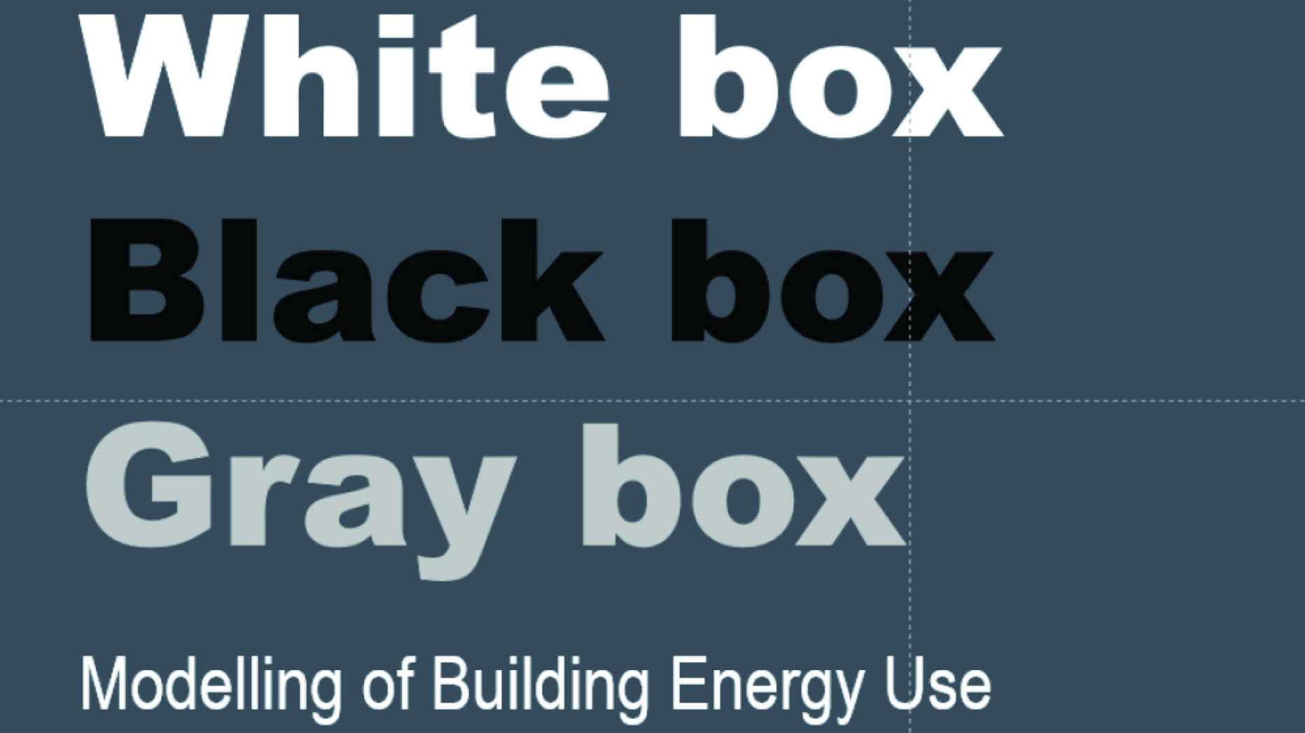
This paper will briefly review the use of white and black models, which are explored in more detail in the sections by Ravi Srinivasan, Pengyuan Shen, and Nancy Ma. The body of the paper will review gray-box methods as they have been applied to buildings
 View Slideshow
